The Impact of International Capital Flows on Oil Price Stability in Algeria
Slimani Abdelwahab
slimaniabdelwahab01@univ-adrar.edu.dz
Ahmed Draia University of Adrar
Received: 09/11/2025 Accepted: 02/02/2026 Published: 25/03/2026
Introduction
Since the beginning of the current decade of the third millennium, the world has experienced a series of health, political, and economic events and phenomena that have had significant repercussions on oil prices. Oil occupies a strategic position in the international economy, as it is considered a valuable commodity due to its scarcity and finite nature, which affects its supply by producing countries.
Russia is among the largest producers of this commodity, ranking third after the United States and Saudi Arabia, with approximately seven million barrels of oil and petroleum products produced daily. Russia’s involvement in the war with Ukraine had a substantial impact on oil prices. The world witnessed an unprecedented surge in oil prices, unseen for the past fourteen years, with prices reaching nearly USD 140 per barrel, compared to around USD 77 per barrel in December 2021.
Although this situation appears beneficial for oil-producing countries such as Algeria, it may discourage the attraction of foreign capital by creating reliance on the currently high oil revenues. Conversely, Algeria may exploit the price differential in oil markets by granting tax and financial incentives to attract international capital and achieve strategic objectives.
Research Problem
In light of the foregoing, the research problem can be formulated as follows:
To what extent do fluctuations in oil prices affect international capital flows?
Sub-questions
The following sub-questions stem from the main problem:
- Is there a relationship between the two variables in the short run?
- Is there a relationship between the two variables in the long run?
- What is the nature of the relationship between oil price fluctuations and international capital flows?
Research Hypotheses
Based on the research problem, sub-questions, and previous studies, the following hypotheses are proposed:
- There is a statistically significant relationship between the two variables under study.
- There is a cointegration relationship between the study variables.
- The relationship is positive; that is, an increase in oil prices leads to greater attraction of international capital.
Previous Studies
Qanouni and Amer (2019): “International Capital Flows and Economic Growth in Algeria: An Empirical Study (1990–2018)”
This study aimed to investigate the relationship between international capital flows in their various forms and economic growth in Algeria during the period 1990–2018. The researchers adopted a descriptive-analytical approach to describe and analyze concepts related to international capital flows and economic growth. They also employed a quantitative econometric approach to assess the impact of capital flows on economic growth using the Autoregressive Distributed Lag (ARDL) model.
The findings revealed the existence of a long-run relationship between foreign direct investment, migrants’ remittances, external debt, foreign aid, and economic growth, with varying effects in the short and long run. The study concluded that Algeria needs deep reforms to attract more foreign capital, particularly through creating a favorable environment that would enable these flows to contribute effectively to economic growth.
Ahlam (2013): “The Impact of Changes in Foreign Exchange Reserve Currency Values on Capital Flows: The Case of Algeria”
This study examined the effect of changes in the value of reserve currencies on capital flows in Algeria using available data. It relied on the historical approach to trace the evolution of capital flows, the descriptive approach to describe phenomena, the analytical approach to analyze tables and statistics, the comparative approach to compare the exchange rates of the euro, the U.S. dollar, and the Algerian dinar, and econometric methods to estimate and model the data.
The study concluded that an increase in the value of reserve currencies leads to an increase in the balance of capital flows in Algeria, and vice versa. It also found that the euro has become the currency exerting the greatest influence on capital flows in Algeria in recent years (since 2007), replacing the U.S. dollar.
Chachoua, Saadaoui, and Amouri (2020): “Impact de la Loi 51%-49% sur l’Attraction de l’Investissement Direct Étranger”
This study investigated the impact of the Algerian government’s adoption of the 49%-51% rule in 2009 on foreign direct investment inflows by analyzing FDI data in Algeria for the period 2005–2015 obtained from the World Bank database. The study employed descriptive and analytical methods.
The results showed that the implementation of this law, in the context of the global economic crisis, had a negative impact on foreign direct investment inflows and constituted an obstacle to the development of FDI in Algeria. Moreover, foreign investors tended to redirect their investments toward neighboring countries that offered a more favorable business climate.
Chapter One: Theoretical Foundations of the Study Variables
Section One: Oil Prices
First: Definition of Oil Price
The oil price refers to the monetary value assigned to petroleum products during a specific period as a result of the interaction of several economic, social, political, and climatic factors, in addition to the prevailing market structure. From this definition, it can be inferred that the oil price is determined by the following components:
- The quantity of oil supplied at a given price;
- The quantity of oil demanded at a given price;
- The structure of the oil market, particularly the degree of competition among producers;
- The availability and quality of information possessed by buyers and sellers, which determine the level of confidence or risk associated with transactions.
Second: Types of Oil Prices
Oil prices can be classified into the following categories:
1. Posted Price
The posted price emerged in the United States in 1830, when oil companies assumed responsibility for announcing prices at production wells immediately after purchasing crude oil from producers. With the expansion of production areas outside the United States, the pricing process shifted from wells to export ports.
2. Official Price
The official price appeared in 1880 when crude oil transactions were conducted at the wellhead. Oil companies announced their prices and reinforced them with discounts, giving rise to price competition. Some economists argue that the official price is determined by the value of refined petroleum products in a competitive final consumption market. Consequently, any change in derived demand directly affects the spot price of crude oil, which in turn influences the official price.
3. Spot Price
Also referred to as the free-market price, the spot price is determined according to market forces of supply and demand. It emerged through the development of the spot market by major oil companies. This market represents a short-term free market in which crude oil is traded outside long-term contracts between producing countries and foreign companies.
4. Reference Price
Oil-producing countries use the reference price to support their revenues. It is generally lower than the posted price but higher than the actual market price. The reference price is calculated based on the official and spot prices over several years.
5. Realized Price
With the emergence of new oil companies that offered various discounts and favorable commercial conditions to buyers, state-owned oil companies adopted similar pricing strategies. This type of pricing became known as the realized price, referring to the actual price at which transactions are completed. It is also called the true or fair price.
6. Tax-Cost Price
This price is adopted by oil companies operating in oil-producing territories. These companies extract oil and purchase it at a price equal to production costs plus the government’s return represented by income taxes. This price is considered the benchmark around which other oil prices fluctuate.
Section Two: Capital Flows
First: Definition of Capital Flows
Capital is one of the principal factors of production and serves as a means for exploiting various economic resources. Since capital is unevenly distributed across countries, reducing these disparities lies at the core of the international monetary system. Capital encompasses not only productive assets but also financial assets such as long- and short-term securities and shares, in addition to tangible assets including machinery, equipment, and real estate.
Second: Forms of Capital Flows
Foreign capital generally flows through the following channels:
- Foreign Direct Investment (FDI);
- Foreign Portfolio Investment (FPI);
- External Loans;
- Foreign Aid and Grants.
Chapter Two: Econometric Analysis of the Impact of Oil Price Fluctuations on International Capital Flows
In this chapter, an econometric model is constructed to examine the impact of oil price fluctuations on capital flows using annual data covering the period 1980–2019, corresponding to 39 observations for each variable. The Vector Autoregression (VAR) model is employed to estimate the relationship between the variables.
First: Study Variables and Data Sources
This study employs a model consisting of two variables. Table 1 presents the source and measurement unit of each variable, along with the expected relationship between them, their symbols in the model, and the study period.
Table 1. Description of the Study Variables
| Variable | Type | Source | Measurement Unit | Symbol in Study | Study Period |
| Oil Prices | Independent Variable | OPEC Official Website | Annual average price of Brent crude oil in U.S. dollars per barrel | OIL | 1980–2019 |
| Capital Flows | Dependent Variable | World Bank Official Website | Percentage of Gross Domestic Product (GDP) | INV | 1980–2019 |
Source: Prepared by the authors.
Descriptive Statistics of the Study Variables
Table 2. Descriptive Statistics of the Study Variables
| Variable | Mean | Standard Deviation | Maximum Value | Minimum Value |
| OIL | 43.32000 | 17.32800 | 111.6300 | 12.80000 |
| INV | 0.643594 | 0.2574376 | 2.033266 | -0.324012 |
Source: Prepared by the authors based on the outputs of EViews 10.
Descriptive Statistics of the Study Variables
As shown in the above table, the average oil price during the study period amounted to USD 43.32 per barrel. The mean value of the capital flows variable reached 64%. The highest value of oil prices was recorded in 2012, reaching USD 111.63 per barrel, while the capital flows variable attained its highest level in 2001.
Regarding the minimum values, the capital flows variable recorded a negative value in 2015, amounting to –32%. This negative value can be interpreted as a net outflow of capital that had previously been invested in the national economy. As for oil prices, the lowest value was recorded in 1998, when the price fell to USD 12.8 per barrel.
Furthermore, the standard deviation of the oil price variable amounted to 1,732.800, indicating a significant degree of variability over the study period. In comparison, the standard deviation of the capital flows variable was estimated at 25.74376.
Second: Stationarity Analysis of the Time Series
It is necessary to verify the stationarity of the time series for all study variables before proceeding with econometric estimation. To detect the presence of unit roots, the Augmented Dickey-Fuller (ADF) test was employed. The results are presented below.
Table 3. Augmented Dickey-Fuller (ADF) Test Results for the Study Variables
| Model Specification | OIL Series at Level | INV Series at Level | OIL Series at First Difference | INV Series at First Difference |
| Intercept | -1.3158 | -2.4841 | -5.5847 | -6.7513 |
| Prob. | 0.6126 | 0.1270 | 0.0000 | 0.0000 |
| Intercept and Trend | -2.1697 | -3.3234 | -5.5130 | -6.6757 |
| Prob. | 0.4924 | 0.0774 | 0.0003 | 0.0000 |
| No Intercept and No Trend | -0.4807 | -1.7331 | -5.6466 | -8.3872 |
| Prob. | 0.5011 | 0.0787 | 0.0000 | 0.0000 |
| Stationarity Test Result | Non-stationary at level; stationary at first difference | Non-stationary at level; stationary at first difference | Stationary at first difference | Stationary at first difference |
Source: Prepared by the authors based on EViews outputs.
According to Table 3, both series are non-stationary at level, indicating the presence of a unit root problem, since the absolute values of the calculated statistics are smaller than the absolute values of the corresponding critical values. However, after taking the first difference, both series became stationary, implying that they are integrated of order one, I(1), whether with an intercept, with an intercept and trend, or without an intercept and trend. In this case, the absolute values of the calculated statistics exceed the corresponding critical values.
The following figure illustrates the time series after first differencing and confirms their stationarity.
Figure 1. Graphical Representation of the Stationary Time Series
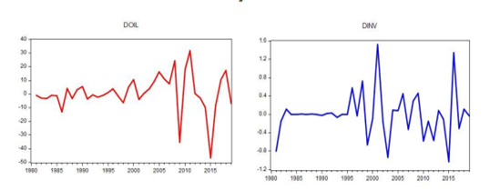
Source: EViews 10 outputs.
Third: Determination of the Optimal Lag Length and Cointegration Test
The stationarity analysis revealed that both study variables are integrated of the same order, namely I(1). According to Granger, this suggests the possibility of a cointegration relationship between the variables. However, before conducting the cointegration test, it is necessary to determine the optimal lag length.
Table 4. Determination of the Optimal Lag Length for the VAR Model
| Lag | LogL | LR | AIC | SC | HQ |
| 0 | -206.4016 | NA | 11.57787 | 11.66584 | 11.60857 |
| 1 | -164.6814 | 76.48693* | 9.482303* | 9.746222* | 9.574418* |
| 2 | -162.0593 | 4.515877 | 9.558851 | 9.998718 | 9.712377 |
| 3 | -159.0846 | 4.792593 | 9.615812 | 10.23162 | 9.830747 |
| 4 | -157.3594 | 2.587816 | 9.742189 | 10.53395 | 10.01853 |
Source: Prepared by the authors based on EViews 10 outputs.
The asterisk (*) indicates the minimum value selected for each lag-order criterion. The test was performed at the 5% significance level.
From the table above, it can be observed that the minimum values of all information criteria correspond to a lag length of one, implying that the optimal number of lags is one (1).
Table 5. Johansen Cointegration Test Results
| Hypothesis (No. of CE(s)) | Trace Statistic | Critical Value (5%) | Prob. |
| None (No cointegrating equation) | 0.281641 | 15.49471 | 0.0507 |
| At most one cointegrating equation | 0.073093 | 3.841466 | 0.0894 |
| Hypothesis (No. of CE(s)) | Max-Eigen Statistic | Critical Value (5%) | Prob. |
| None (No cointegrating equation) | 0.281641 | 14.26460 | 0.0910 |
| At most one cointegrating equation | 0.073093 | 3.841466 | 0.0894 |
Source: Prepared by the authors based on EViews 10 outputs.
The results in Table 5 indicate that the Johansen statistics for all hypotheses are greater than their corresponding critical values at the 5% significance level. Consequently, the null hypothesis is accepted, implying the absence of a long-run cointegration relationship between the variables. Therefore, the relationship between these variables should be estimated in the short run using the Vector Autoregression (VAR) model, since the Error Correction Model (ECM) cannot be employed in the absence of a long-run equilibrium relationship between the study variables.
Fourth: Estimation of the VAR(1) Model
After confirming that both series are stationary at first differences, determining the optimal lag length, and establishing the absence of cointegration among the variables, the autoregressive relationship between oil prices (OIL) and capital flows (INV) is estimated.
Table 6. Estimation of the VAR Model
Source: Prepared by the authors based on EViews 10 outputs.
1. Statistical Analysis
To verify both the significance of the parameters and the overall significance of the model, the autoregressive equation was estimated using the Ordinary Least Squares (OLS) method. The estimation results are presented in the following table.
Table 7. Estimation of the VAR(1) Model Using the OLS Method
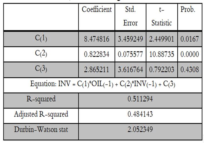
Source: Prepared by the authors based on EViews 10 outputs.
From the above table, it is evident that the model as a whole is statistically significant. The calculated F-statistic is 18.83192, which exceeds the corresponding critical value. Therefore, the alternative hypothesis is accepted, indicating that the model is globally significant.
Regarding partial significance, the coefficient associated with oil prices is statistically significant, as the p-value corresponding to the Student’s t-statistic equals 0.0167, which is lower than the significance threshold of 0.05. Similarly, the coefficient associated with capital flows is statistically significant, with a p-value of 0.0000. In contrast, the constant term is found to be statistically insignificant.
Furthermore, the coefficient of determination is R² = 0.51, indicating that the independent variable explains 51% of the variation in capital flows, while the remaining 49% is attributable to other variables or factors not included in the model.
The Durbin-Watson statistic (DW) equals 2.05, suggesting that the residuals are free from autocorrelation, as this value is very close to 2. To further verify the stability of the model, the inverse roots test is conducted.
Figure 2. Structural Stability Test of the VAR(1) Model
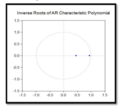
Source: EViews 10 outputs.
Since model instability may lead to inaccurate and misleading results, conducting this test is essential. As illustrated in Figure 2, all inverse roots are less than one and lie within the unit circle. Therefore, the VAR(1) model is considered stable, confirming the structural stability of the estimated Vector Autoregression model.
2. Economic Interpretation
Based on the estimation results of the Vector Autoregression (VAR) model, and after verifying the statistical significance of the parameters and the adequacy of the model in explaining changes in capital flows as a function of oil price fluctuations, the following conclusions can be drawn:
- In this model, capital flows are explained by their first lag, the first lag of oil prices, and the constant term. In other words, capital flows in year ttt are influenced by capital flows and oil price fluctuations in year t−1t-1t−1.
- Current capital flows are positively affected by capital flows in the previous year. According to Table 7, the estimated coefficient is:
b=0.700191b = 0.700191b=0.700191
This implies that an increase in capital flows in the previous year is expected to be followed by a further increase in the subsequent year, and vice versa. This finding reflects the well-known saying that “capital is cowardly,” meaning that investors generally prefer projects and markets that have already demonstrated favorable investment conditions in order to minimize risk. Consequently, investors tend to direct their funds toward regions that have previously experienced strong capital inflows.
- Capital flows in period ttt are also positively affected by oil price fluctuations in period t−1t-1t−1. According to Table 7, the estimated coefficient is:
b=0.000696
This result is expected because higher oil prices provide the government with greater financial resources, enabling it to improve infrastructure, grant tax exemptions and incentives to existing investors, and enact laws and regulations designed to attract both domestic and foreign investment. Such measures stimulate potential investors and encourage current investors to expand their activities.
Fifth: Causality Analysis Between the Study Variables
At this stage, the direction of causality between oil price fluctuations and capital flows is examined using the Granger Causality Test.
Table 8. Granger Causality Test Results
Source: Prepared by the authors based on EViews 10 outputs.
The results presented in the table indicate that oil prices do not Granger-cause capital flows, and likewise, capital flows do not Granger-cause oil price fluctuations. This conclusion is supported by the probability values, which are greater than the 5% significance level, leading to the acceptance of the null hypothesis.
Therefore, there is no causality running in either direction between the two variables. It can thus be concluded that oil prices and capital flows are not linked by a long-run causal relationship in the Algerian economy during the study period.
Sixth: Impulse Response Functions
Impulse response analysis helps reveal the interactions and dynamic relationships among the variables under study. In this research, emphasis is placed on introducing shocks to oil prices and measuring their transmission to the dependent variable.
Generally, shocks are considered temporary, since both variables eventually return to their long-run equilibrium levels, as illustrated by the impulse response functions shown below. This provides further evidence of the stability of the VAR model.
Figure 3. Impulse Response Functions
Source: EViews 10 outputs.
From the figure, it can be concluded that:
Based on the impulse response estimates over a ten-year horizon, a one-standard-deviation shock to oil prices exerts a positive effect on capital flows. However, this effect begins to weaken after the fourth year and gradually declines until the tenth year.
Conclusion
The present study reveals that the relationship between oil prices and capital flows is positive in the short run. Specifically, increases in oil prices are accompanied by greater inflows of foreign capital. These findings confirm the first and third hypotheses while rejecting the second hypothesis.
Study Findings
The study yielded the following results:
- The estimated relationship between oil prices and capital flows is economically and statistically acceptable.
- The two time series are integrated of the same order, I(1). Cointegration tests reveal the absence of a long-run equilibrium relationship between the variables.
- Oil price fluctuations explain approximately 51% of the variations in capital flows, while the remaining 49% is attributable to other variables and factors not included in the model.
- No causal relationship exists between the two variables.
- A shock to oil prices initially leads to an increase in capital flows. However, this effect gradually diminishes over the medium and long term, with the variables returning to their previous levels after approximately ten years.
References
- Chachoua, A., Saadaoui, M. M., & Amouri, I. (2020). Impact de la Loi 51%-49% sur l’attraction de l’investissement direct étranger. Future Economic Scientific Journal, 1(1), 245–260.
- Bouchrit, O. (2014). The Role of Monetary Policy in Achieving Macroeconomic Equilibrium. Master’s Thesis.
- Ben Zidane Hadj. (2005/2006). The Impact of Oil Price Changes on Economic Growth. Unpublished Master’s Thesis, Faculty of Economics, Commercial Sciences, and Management Sciences, University of Mostaganem, Algeria.
- Baghdad, B. (2008/2009). An Econometric Modeling of Algerian Oil Prices: The Case of Saharan Blend (2006–2009). Unpublished Master’s Thesis, Faculty of Economics and Management Sciences, Quantitative Economics Specialization, University of Algiers 3, Algeria.
- Qanouni, H., & Amer, A. (2019). International Capital Flows and Economic Growth in Algeria: An Empirical Study (1990–2018). Organisation et Travail Review, 8(3), 111–124.
- Hariri, A. G. (2010). The Effects of Foreign Capital Flows and Policies to Address Their Risks. North African Economies Journal, 43–64.
- Kabli, Z. (1999). Determining Crude Oil Prices in the Short and Long Run Using Cointegration and Error Correction Models. Unpublished Master’s Thesis, Faculty of Economics and Management Sciences, University of Algiers, Algeria.
- Lashlah, A. (2013). The Impact of Changes in Foreign Exchange Reserve Currency Values on Capital Flows: The Case of Algeria. Master’s Thesis.
Top of Form